6. Examples
Examples of different uses of PyIOmica package API.
A Jupyter notebook with all examples is available at: https://github.com/gmiaslab/pyiomica/tree/master/docs/examples
Enrichment report
Function ExportEnrichmentReport generates enrichment report in form of “.xlsx” file.
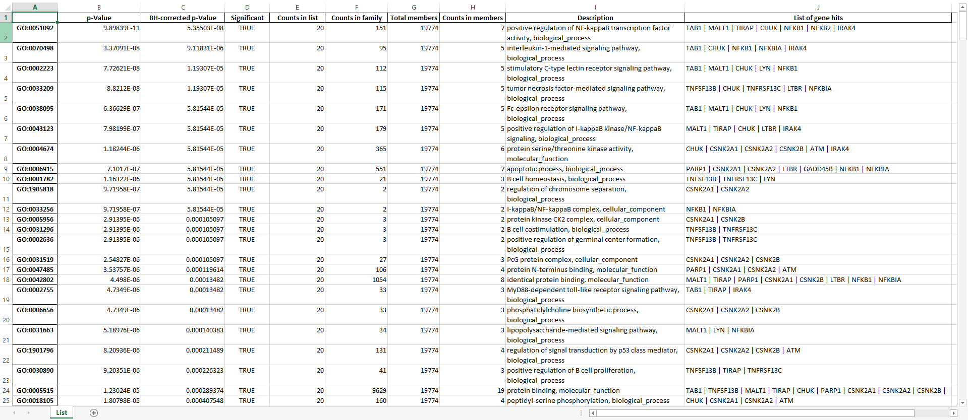
The are following columns in each Worksheet of the output “.xlsx” file
ID: Annotation term identifier
p-Value: Probability to find at least “Counts in members” number of genes when drawing “Counts in list” genes “Counts in family” times (without replacement) from “Counts in members” identifiers. Note: this is the behavior when using default setting, i.e. Hypergeometric distribution testing function
BH-corrected p-Value: p-Value corrected for false discovery rate (FDR) via Benjamini-Hochberg procedure
Significant: Whether the “BH-corrected p-Value” is below the threshold (typically 0.05) specified for the enrichment analysis
Counts in list: Number of genes in the input list
Counts in family: Number of genes in a particular annotation term
Total members: Number of members (e.g. UniprotIDs) in the IDs to annotation terms dictionary
Counts in members: Number of annotation terms in which at least of gene from the input list appear
Description: Description of a particular annotation term, e.g. details/type
List of gene hits: Gene identifiers that are found in a particular annotation term. The identifiers are separated by a Vertical bar
Import of MathIOmica Objects
#import sys
#sys.path.append("../..")

import pyiomica as pio

from pyiomica.utilityFunctions import readMathIOmicaData

print(pio.ConstantPyIOmicaExamplesDirectory, '\n')
tempPath = pio.os.path.join(pio.ConstantPyIOmicaExamplesDirectory, 'MathIOmicaExamples')

rnaExample = readMathIOmicaData(pio.os.path.join(tempPath, 'rnaExample'))
print('rnaExample:', str(rnaExample)[:400], '\t. . .\n')

proteinClassificationExample = readMathIOmicaData(pio.os.path.join(tempPath, 'proteinClassificationExample'))
print('proteinClassificationExample:', str(proteinClassificationExample)[:400], '\t. . .\n')

proteinTimeSeriesExample = readMathIOmicaData(pio.os.path.join(tempPath, 'proteinTimeSeriesExample'))
print('proteinTimeSeriesExample:', str(proteinTimeSeriesExample)[:400], '\t. . .\n')

proteinExample = readMathIOmicaData(pio.os.path.join(tempPath, 'proteinExample'))
print('proteinExample:', str(proteinExample)[:400], '\t. . .\n')

metabolomicsPositiveModeExample = readMathIOmicaData(pio.os.path.join(tempPath, 'metabolomicsPositiveModeExample'))
print('metabolomicsPositiveModeExample:', str(metabolomicsPositiveModeExample)[:400], '\t. . .\n')

metabolomicsNegativeModeExample = readMathIOmicaData(pio.os.path.join(tempPath, 'metabolomicsNegativeModeExample'))
print('metabolomicsNegativeModeExample:', str(metabolomicsNegativeModeExample)[:400], '\t. . .\n')
Clustering object export example
Example of a clustering object exported to “.xlsx” file.
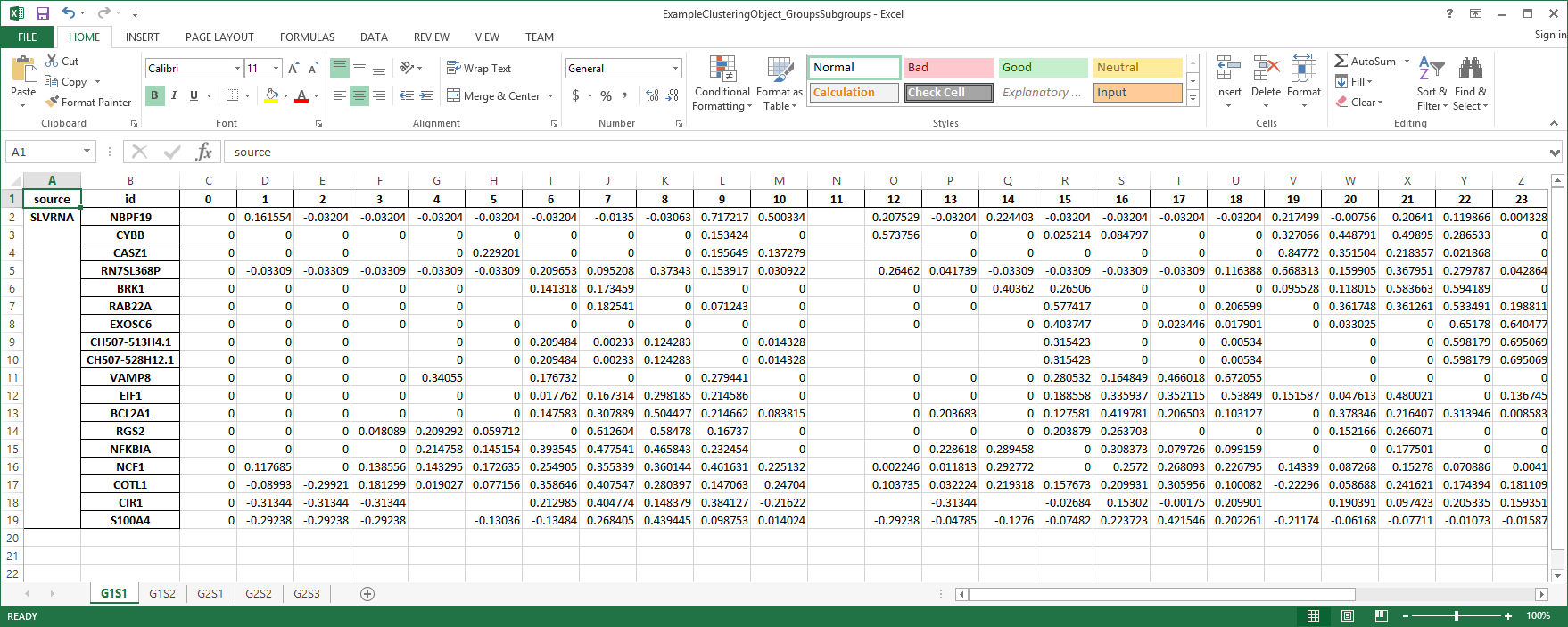
The file contains one Spreadsheet for each subgroup in a clustering object. The spreadsheet is structrured as follows. The first column indicates the data source, the second column has gene identifiers, all the remaining colummns contain data and autocorrelations. Note, this is the structure when using the default settings. User can modify output by setting various options.
GO Analysis examples
#import sys
#sys.path.append("../..")

import pyiomica as pio

from pyiomica.enrichmentAnalyses import GOAnalysis, ExportEnrichmentReport
from pyiomica import dataStorage as ds

EnrichmentOutputDirectory = 'results/EnrichmentOutputDirectory/'

#Let's do a GO analysis for a group of genes, annotated with their "Gene Symbol":
goExample1 = GOAnalysis(["TAB1", "TNFSF13B", "MALT1", "TIRAP", "CHUK",
                                "TNFRSF13C", "PARP1", "CSNK2A1", "CSNK2A2", "CSNK2B", "LTBR",
                                "LYN", "MYD88", "GADD45B", "ATM", "NFKB1", "NFKB2", "NFKBIA",
                                "IRAK4", "PIAS4", "PLAU"])

ExportEnrichmentReport(goExample1, AppendString='goExample1', OutputDirectory=EnrichmentOutputDirectory + 'GOAnalysis/')

#The information can be computed for multiple groups, if these are provided as an association:
analysisGOAssociation = GOAnalysis({"Group1": ["C6orf57", "CD46", "DHX58", "HMGB3", "MAP3K5", "NFKB2", "NOS2", "PYCARD", "PYDC1", "SSC5D"],
                                                "Group2": ["TAB1", "TNFSF13B", "MALT1", "TIRAP", "CHUK", "TNFRSF13C", "PARP1", "CSNK2A1", "CSNK2A2", "CSNK2B", "LTBR",
                                                            "LYN", "MYD88", "GADD45B", "ATM", "NFKB1", "NFKB2", "NFKBIA", "IRAK4", "PIAS4", "PLAU"]})

ExportEnrichmentReport(analysisGOAssociation, AppendString='analysisGOAssociation', OutputDirectory=EnrichmentOutputDirectory + 'GOAnalysis/')

#The data can be computed with or without a label. If labeled, the gene ID must be the first element for each ID provided. The data is in the form {ID,label}:
analysisGOLabel = GOAnalysis([["C6orf57", "Protein"], ["CD46", "Protein"], ["DHX58", "Protein"], ["HMGB3", "Protein"], ["MAP3K5", "Protein"],
                                        ["NFKB2", "Protein"], ["NOS2", "Protein"], ["PYCARD", "Protein"], ["PYDC1","Protein"], ["SSC5D", "Protein"]])

ExportEnrichmentReport(analysisGOLabel, AppendString='analysisGOLabel', OutputDirectory=EnrichmentOutputDirectory + 'GOAnalysis/')

#The data can be mixed, e.g. proteins and RNA with different labels:
analysisGOMixed = GOAnalysis([["C6orf57", "Protein"], ["CD46", "Protein"], ["DHX58", "Protein"], ["HMGB3", "RNA"], ["HMGB3", "Protein"], ["MAP3K5", "Protein"],
                                        ["NFKB2", "RNA"], ["NFKB2", "Protein"], ["NOS2", "RNA"], ["PYCARD", "RNA"], ["PYDC1", "Protein"], ["SSC5D", "Protein"]])

ExportEnrichmentReport(analysisGOMixed, AppendString='analysisGOMixed', OutputDirectory=EnrichmentOutputDirectory + 'GOAnalysis/')

#We can instead treat the data as different by setting the MultipleList and MultipleListCorrection options:
analysisGOMixedMulti = GOAnalysis([["C6orf57", "Protein"], ["CD46", "Protein"], ["DHX58", "Protein"], ["HMGB3", "RNA"], ["HMGB3", "Protein"], ["MAP3K5", "Protein"],
                                            ["NFKB2", "RNA"], ["NFKB2", "Protein"], ["NOS2", "RNA"], ["PYCARD", "RNA"], ["PYDC1", "Protein"], ["SSC5D", "Protein"]],
                                            MultipleList=True, MultipleListCorrection='Automatic')

ExportEnrichmentReport(analysisGOMixedMulti, AppendString='analysisGOMixedMulti', OutputDirectory=EnrichmentOutputDirectory + 'GOAnalysis/')

#Enrichment analysis function GOAnalysis can be used with a clustering object.
#First run examples of use of categorization functions to generate clustering objects.
#Then run "results = GOAnalysis(ds.read(pathToClusteringObjectOfInterest))",
#to calculate enrichment for each group in each class, and then export enrichment results to a file if necesary.
KEGG Analysis examples
#import sys
#sys.path.append("../..")

import pyiomica as pio

from pyiomica.enrichmentAnalyses import KEGGAnalysis, ExportEnrichmentReport
from pyiomica import dataStorage as ds

EnrichmentOutputDirectory = pio.os.path.join('results', 'EnrichmentOutputDirectory', '')

#Let's do a KEGG pathway analysis for a group of genes (most in the NFKB pathway), annotated with their "Gene Symbol":
keggExample1 = KEGGAnalysis(["TAB1", "TNFSF13B", "MALT1", "TIRAP", "CHUK", "TNFRSF13C", "PARP1", "CSNK2A1", "CSNK2A2", "CSNK2B", "LTBR", "LYN", "MYD88",
                                        "GADD45B", "ATM", "NFKB1", "NFKB2", "NFKBIA", "IRAK4", "PIAS4", "PLAU", "POLR3B", "NME1", "CTPS1", "POLR3A"])

ExportEnrichmentReport(keggExample1, AppendString='keggExample1', OutputDirectory=EnrichmentOutputDirectory + 'KEGGAnalysis/')

#The information can be computed for multiple groups, if these are provided as an association:
analysisKEGGAssociation = KEGGAnalysis({"Group1": ["C6orf57", "CD46", "DHX58", "HMGB3", "MAP3K5", "NFKB2", "NOS2", "PYCARD", "PYDC1", "SSC5D"],
                                                    "Group2": ["TAB1", "TNFSF13B", "MALT1", "TIRAP", "CHUK", "TNFRSF13C", "PARP1", "CSNK2A1", "CSNK2A2", "CSNK2B", "LTBR",
                                                "LYN", "MYD88", "GADD45B", "ATM", "NFKB1", "NFKB2", "NFKBIA", "IRAK4", "PIAS4", "PLAU", "POLR3B", "NME1", "CTPS1", "POLR3A"]})

ExportEnrichmentReport(analysisKEGGAssociation, AppendString='analysisKEGGAssociation', OutputDirectory=EnrichmentOutputDirectory + 'KEGGAnalysis/')

#The data can be computed with or without a label. If labeled, the gene ID must be the first element for each ID provided. The data is in the form {ID,label}:
analysisKEGGLabel = KEGGAnalysis([["C6orf57", "Protein"], ["CD46", "Protein"], ["DHX58", "Protein"], ["HMGB3", "Protein"], ["MAP3K5", "Protein"],
                                            ["NFKB2", "Protein"], ["NOS2", "Protein"], ["PYCARD", "Protein"], ["PYDC1","Protein"], ["SSC5D", "Protein"]])

ExportEnrichmentReport(analysisKEGGLabel, AppendString='analysisKEGGLabel', OutputDirectory=EnrichmentOutputDirectory + 'KEGGAnalysis/')

#The same result is obtained if IDs are enclosed in list brackets:
analysisKEGGNoLabel = KEGGAnalysis([["C6orf57"], ["CD46"], ["DHX58"], ["HMGB3"], ["MAP3K5"], ["NFKB2"], ["NOS2"], ["PYCARD"], ["PYDC1"], ["SSC5D"]])

ExportEnrichmentReport(analysisKEGGNoLabel, AppendString='analysisKEGGNoLabel', OutputDirectory=EnrichmentOutputDirectory + 'KEGGAnalysis/')

#The same result is obtained if IDs are input as strings:
analysisKEGGstrings = KEGGAnalysis(["C6orf57", "CD46", "DHX58", "HMGB3", "MAP3K5", "NFKB2", "NOS2", "PYCARD", "PYDC1", "SSC5D"])

ExportEnrichmentReport(analysisKEGGstrings, AppendString='analysisKEGGstrings', OutputDirectory=EnrichmentOutputDirectory + 'KEGGAnalysis/')

#The data can be mixed, e.g. proteins and RNA with different labels:
analysisKEGGMixed = KEGGAnalysis([["C6orf57", "Protein"], ["CD46", "Protein"], ["DHX58", "Protein"], ["HMGB3", "RNA"], ["HMGB3", "Protein"], ["MAP3K5", "Protein"],
                                            ["NFKB2", "RNA"], ["NFKB2", "Protein"], ["NOS2", "RNA"], ["PYCARD", "RNA"], ["PYDC1", "Protein"], ["SSC5D", "Protein"]])

ExportEnrichmentReport(analysisKEGGMixed, AppendString='analysisKEGGMixed', OutputDirectory=EnrichmentOutputDirectory + 'KEGGAnalysis/')

#The data in this case treated as originating from a single population. Protein and RNA labeled data for the same identifier are treated as equivalent.
#We can instead treat the data as different by setting the MultipleList and MultipleListCorrection options:
analysisKEGGMixedMulti = KEGGAnalysis([["C6orf57", "Protein"], ["CD46", "Protein"], ["DHX58", "Protein"], ["HMGB3", "RNA"], ["HMGB3", "Protein"], ["MAP3K5", "Protein"],
                                                ["NFKB2", "RNA"], ["NFKB2", "Protein"], ["NOS2", "RNA"], ["PYCARD", "RNA"], ["PYDC1", "Protein"], ["SSC5D", "Protein"]],
                                                MultipleList=True, MultipleListCorrection='Automatic')

ExportEnrichmentReport(analysisKEGGMixedMulti, AppendString='analysisKEGGMixedMulti', OutputDirectory=EnrichmentOutputDirectory + 'KEGGAnalysis/')

#We can carry out a "Molecular" analysis for compound data. We consider the following metabolomics data, which has labels "Meta"
#and additional mass and retention time information in the form {identifier,mass, retention time, label}:
compoundsExample = [["cpd:C19691", 325.2075, 10.677681, "Meta"], ["cpd:C17905", 594.2002, 8.727458, "Meta"],["cpd:C09921", 204.0784, 12.3909445, "Meta"],
                    ["cpd:C18218", 272.2356, 13.473582, "Meta"], ["cpd:C14169", 235.1573, 12.267084, "Meta"],["cpd:C14245", 262.2296, 13.545572, "Meta"],
                    ["cpd:C09137", 352.2615, 14.0554285, "Meta"], ["cpd:C09674", 296.1624, 12.147417, "Meta"], ["cpd:C00449", 276.1334, 11.004139, "Meta"],
                    ["cpd:C02999", 364.1497, 12.147243, "Meta"], ["cpd:C07915", 309.194, 7.3625283, "Meta"],["cpd:C08760", 496.2309, 8.7241125, "Meta"],
                    ["cpd:C14549", 276.0972, 11.078914, "Meta"], ["cpd:C20533", 601.3378, 12.75722, "Meta"], ["cpd:C20790", 212.1051, 7.127666, "Meta"],
                    ["cpd:C09137", 352.2613, 12.869867, "Meta"], ["cpd:C17648", 400.2085, 10.843841, "Meta"], ["cpd:C07807", 240.1471, 0.48564285, "Meta"],
                    ["cpd:C08564", 324.0948, 10.281, "Meta"], ["cpd:C19426", 338.2818, 13.758765, "Meta"], ["cpd:C02943", 468.3218, 14.263261, "Meta"],
                    ["cpd:C04882", 1193.342, 14.707576, "Meta"]]

compoundsExampleKEGG = KEGGAnalysis(compoundsExample, FilterSignificant=True, AnalysisType='Molecular')

ExportEnrichmentReport(compoundsExampleKEGG, AppendString='compoundsExampleKEGG', OutputDirectory=EnrichmentOutputDirectory + 'KEGGAnalysis/')

#We can carry out multiomics data analysis. We consider the following simple example:
multiOmicsData = [["C6orf57", "Protein"], ["CD46", "Protein"], ["DHX58", "Protein"], ["HMGB3", "RNA"], ["HMGB3", "Protein"],
                    ["MAP3K5", "Protein"], ["NFKB2", "RNA"], ["NFKB2", "Protein"], ["NOS2", "RNA"], ["PYCARD", "RNA"], ["PYDC1", "Protein"],
                    ["SSC5D", "Protein"], ["cpd:C19691", 325.2075, 10.677681, "Meta"], ["cpd:C17905", 594.2002, 8.727458, "Meta"],
                    ["cpd:C09921", 204.0784, 12.3909445, "Meta"], ["cpd:C18218", 272.2356, 13.473582, "Meta"],
                    ["cpd:C14169", 235.1573, 12.267084, "Meta"], ["cpd:C14245", 262.2296, 13.545572, "Meta"],
                    ["cpd:C09137", 352.2615, 14.0554285, "Meta"], ["cpd:C09674", 296.1624, 12.147417, "Meta"],
                    ["cpd:C00449", 276.1334, 11.004139, "Meta"],["cpd:C02999", 364.1497, 12.147243, "Meta"],
                    ["cpd:C07915", 309.194, 7.3625283, "Meta"],["cpd:C08760", 496.2309, 8.7241125, "Meta"],
                    ["cpd:C14549", 276.0972, 11.078914, "Meta"],["cpd:C20533", 601.3378, 12.75722, "Meta"],
                    ["cpd:C20790", 212.1051, 7.127666, "Meta"], ["cpd:C09137", 352.2613, 12.869867, "Meta"],
                    ["cpd:C17648", 400.2085, 10.843841, "Meta"], ["cpd:C07807", 240.1471, 0.48564285, "Meta"],
                    ["cpd:C08564", 324.0948, 10.281, "Meta"], ["cpd:C19426", 338.2818, 13.758765, "Meta"],
                    ["cpd:C02943", 468.3218, 14.263261, "Meta"], ["cpd:C04882", 1193.342, 14.707576, "Meta"]]

#We can carry out "Genomic" and "Molecular" analysis concurrently by setting AnalysisType = "All":
multiOmicsDataKEGG = KEGGAnalysis(multiOmicsData, AnalysisType='All', MultipleList=True, MultipleListCorrection='Automatic')

ExportEnrichmentReport(multiOmicsDataKEGG, AppendString='multiOmicsDataKEGG', OutputDirectory=EnrichmentOutputDirectory + 'KEGGAnalysis/')

#Enrichment analysis function KEGGAnalysis can be used with a clustering object.
#First run examples of use of categorization functions to generate clustering objects.
#Then run "results = KEGGAnalysis(ds.read(pathToClusteringObjectOfInterest))",
#to calculate enrichment for each group in each class, and then export enrichment results to a file if necesary.
Reactome Analysis examples
#import sys
#sys.path.append("../..")

import pyiomica as pio
from pyiomica.enrichmentAnalyses import ReactomeAnalysis, ExportReactomeEnrichmentReport
from pyiomica import dataStorage as ds

EnrichmentOutputDirectory = pio.os.path.join('results', 'EnrichmentOutputDirectory', '')

#Let's do a Reactome analysis for a group of genes, annotated with their "Gene Symbol":
ReactomeExample1 = ReactomeAnalysis(["TAB1", "TNFSF13B", "MALT1", "TIRAP", "CHUK",
                        "TNFRSF13C", "PARP1", "CSNK2A1", "CSNK2A2", "CSNK2B", "LTBR",
                        "LYN", "MYD88", "GADD45B", "ATM", "NFKB1", "NFKB2", "NFKBIA",
                        "IRAK4", "PIAS4", "PLAU"])

ExportReactomeEnrichmentReport(ReactomeExample1,
                               AppendString='ReactomeExample1',
                               OutputDirectory=EnrichmentOutputDirectory + 'ReactomeAnalysis/')

#The information can be computed for multiple groups, if these are provided as an association:
analysisReactomeAssociation = ReactomeAnalysis({"Group1": ["C6orf57", "CD46", "DHX58", "HMGB3", "MAP3K5", "NFKB2", "NOS2", "PYCARD", "PYDC1", "SSC5D"],
                                    "Group2": ["TAB1", "TNFSF13B", "MALT1", "TIRAP", "CHUK", "TNFRSF13C", "PARP1", "CSNK2A1", "CSNK2A2", "CSNK2B", "LTBR", "LYN", "MYD88", "GADD45B", "ATM", "NFKB1", "NFKB2", "NFKBIA", "IRAK4", "PIAS4", "PLAU"]})

ExportReactomeEnrichmentReport(analysisReactomeAssociation,
                               AppendString='analysisReactomeAssociation',
                               OutputDirectory=EnrichmentOutputDirectory + 'ReactomeAnalysis/')

#Enrichment analysis function ReactomeAnalysis can be used with a clustering object.
#First run examples of use of categorization functions to generate clustering objects.
#Then run "results = ReactomeAnalysis(ds.read(pathToClusteringObjectOfInterest))",
#to calculate enrichment for each group in each class, and then export enrichment results to a file if necesary using ExportReactomeEnrichmentReport function.
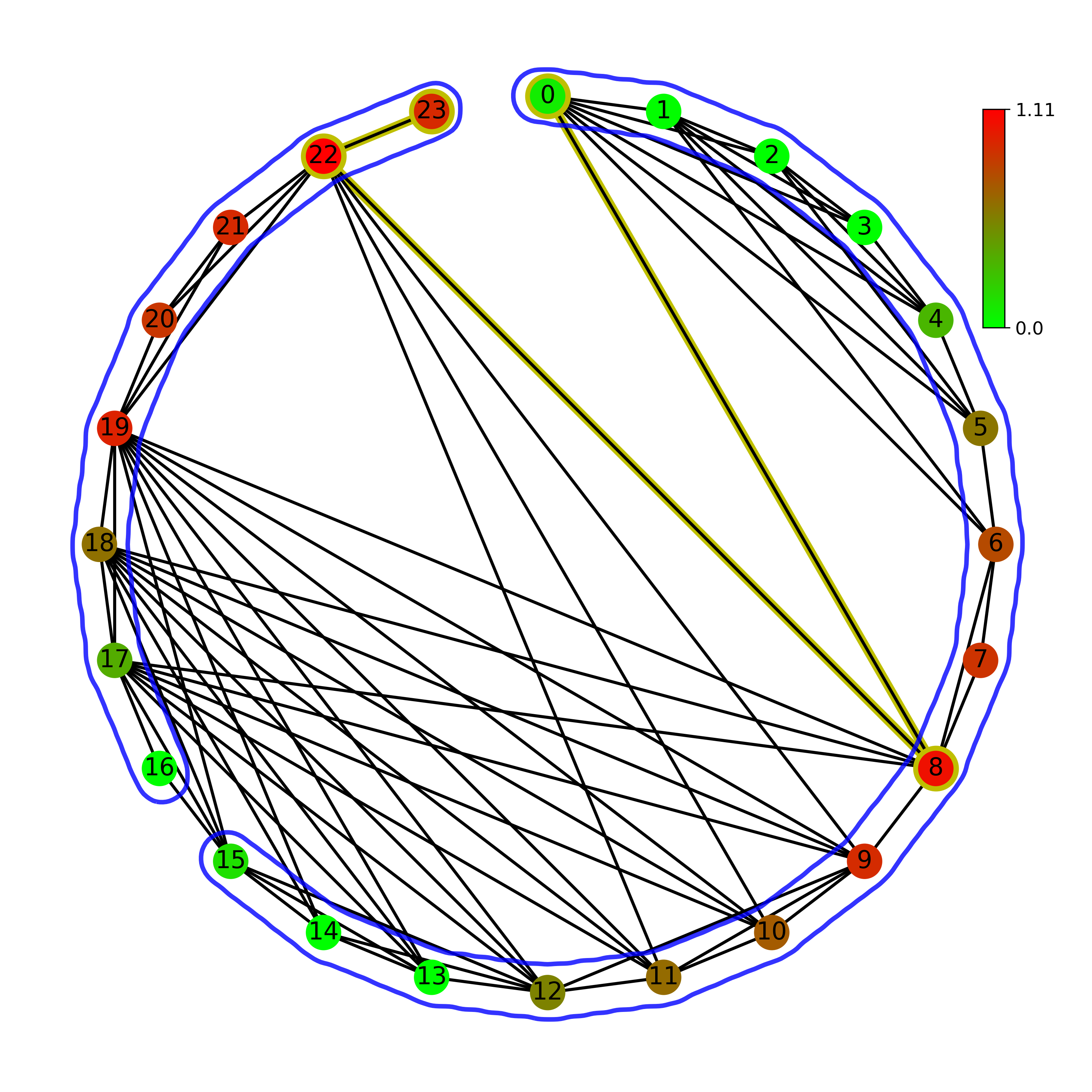
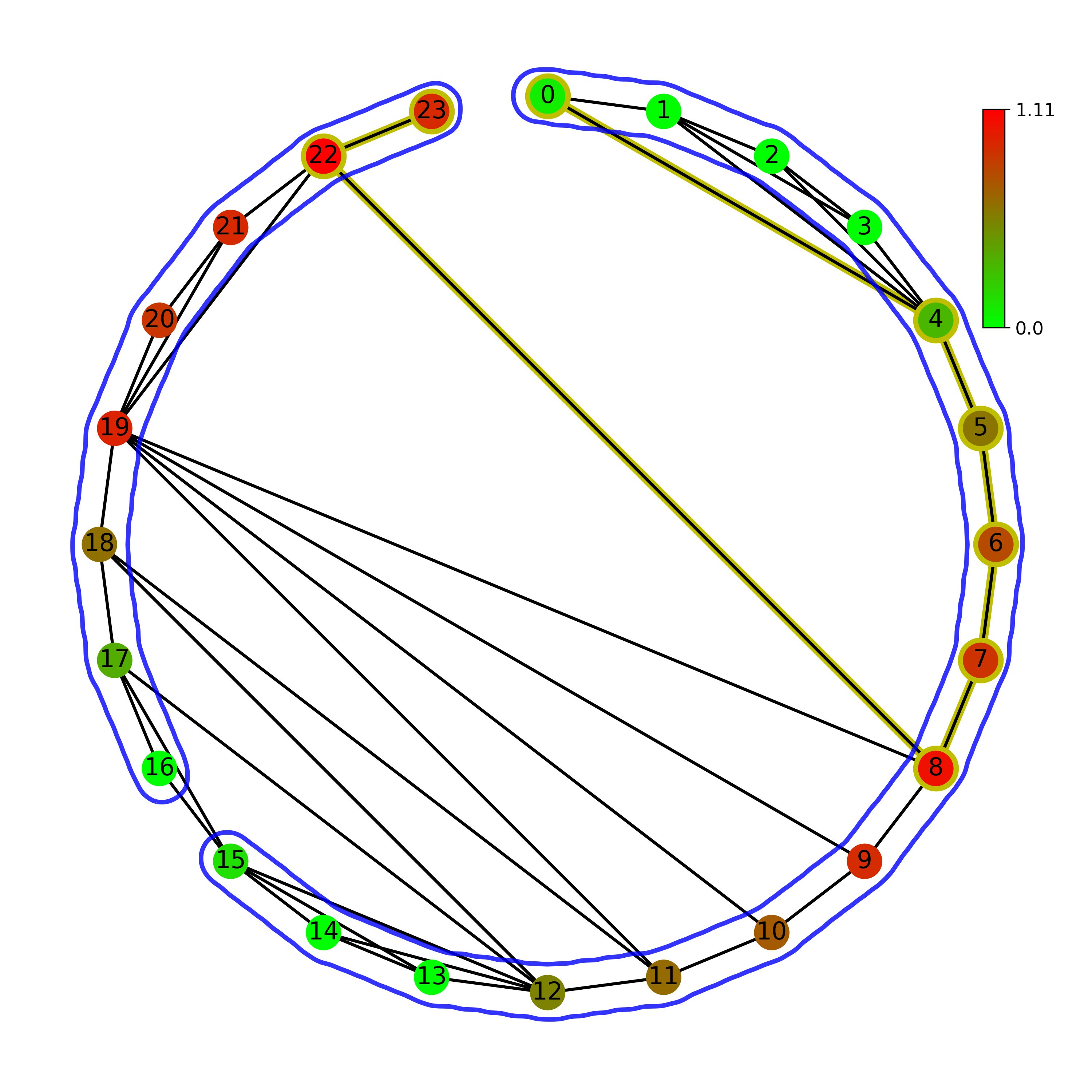
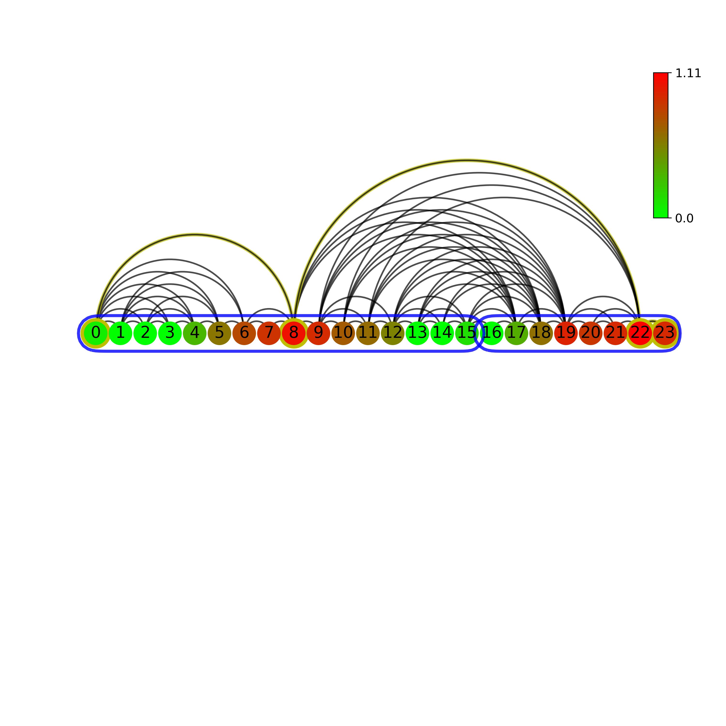
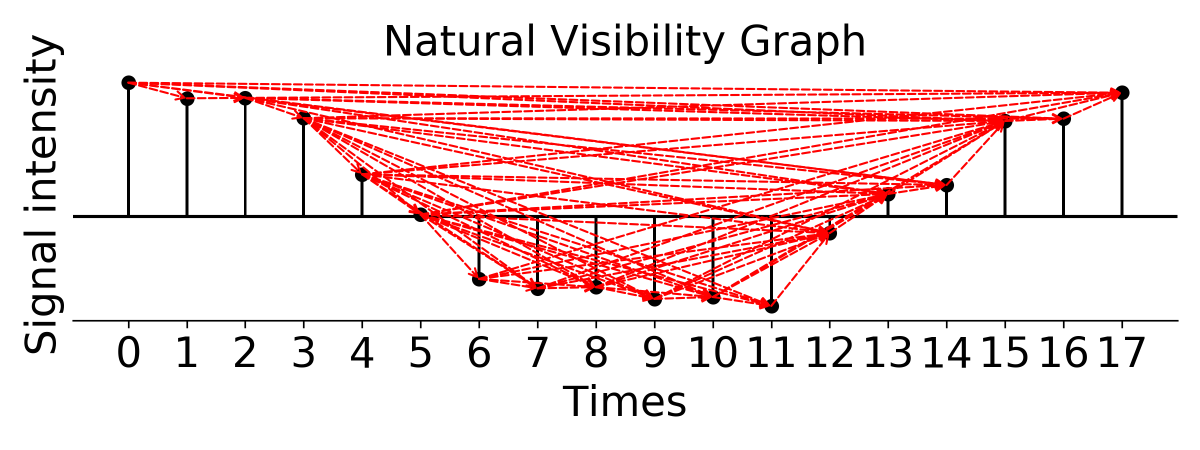
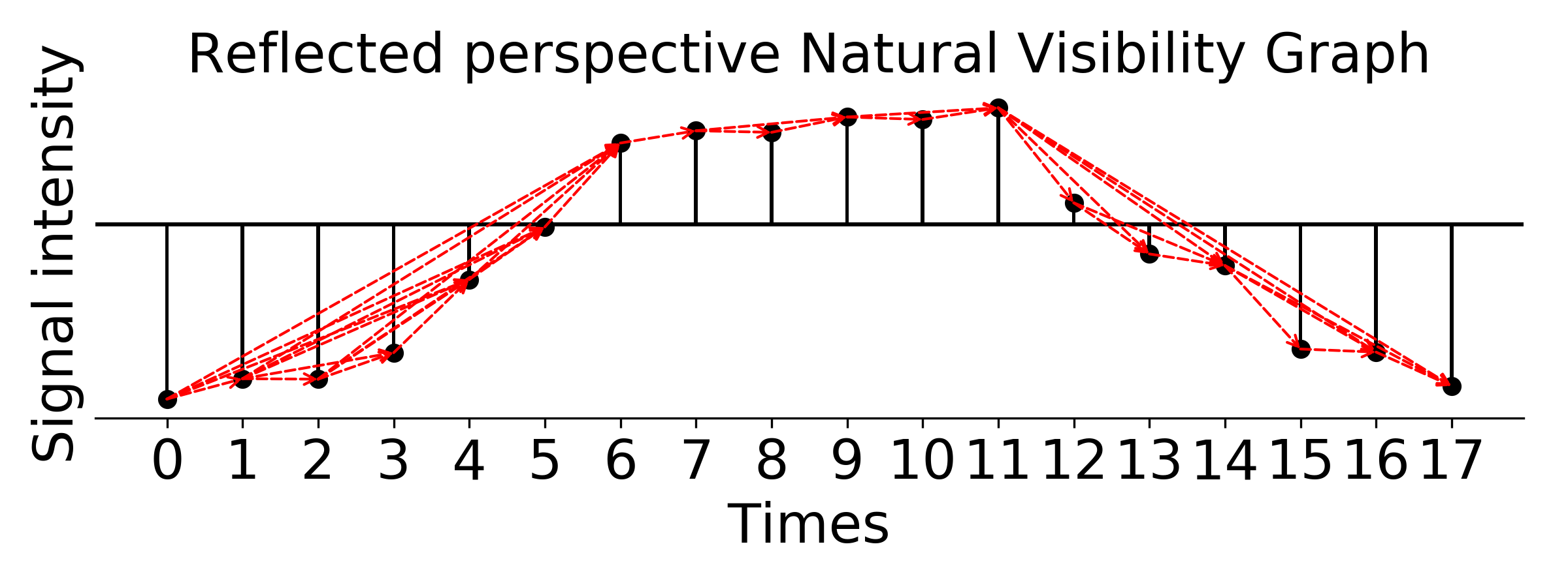
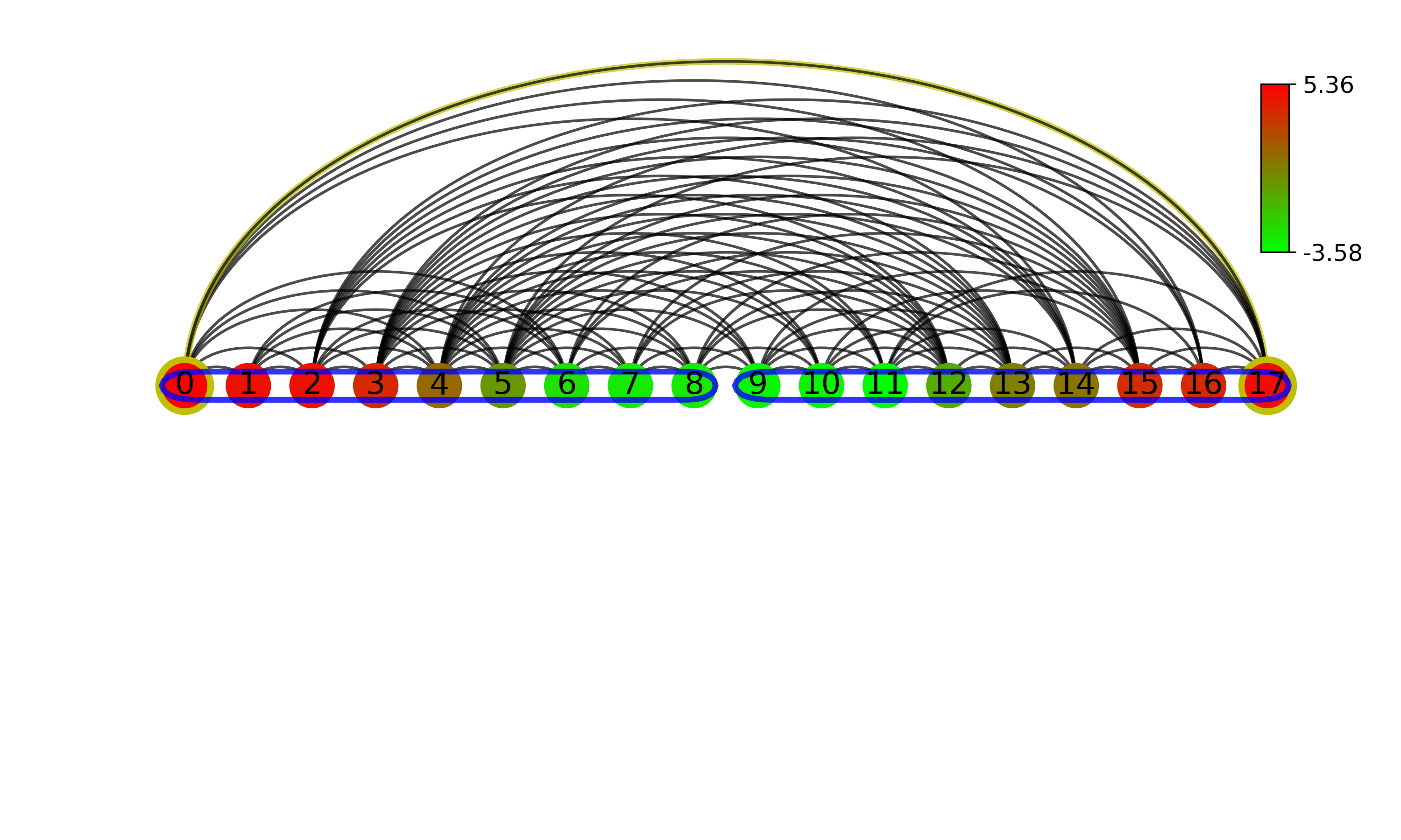
Visibility Graph examples
We represent each timepoint in a series as a node. Temporal events are detected and indicated with solid blue lines encompassing groups of points, or communities. The shortest path identifies nodes (i.e. timepoints) that display high intensity, and thus dominate the global signal profile, are robust to noise, and are likely drivers of the global temporal behavior.
Representing the intensities as bars, this is equivalent to connecting the top of each bar to another top if there is a direct line-of-sight to that top. The resulting visibility graph has characteristics that reflect the equivalent time series temporal structure and can be used to identify trends.
#import sys
#sys.path.append("../..")

import pyiomica as pio

from pyiomica.visualizationFunctions import makeVisibilityGraph, makeVisibilityBarGraph
from pyiomica import dataStorage as ds
from pyiomica.extendedDataFrame import DataFrame

# Make an example of time series
# Set intensities of all signals and the measurement time points (here positions)
positions = pio.np.array(range(24))
intensities = pio.np.cos(pio.np.array(range(24))*0.25 + 1.)**2 + 0.5*(pio.np.random.random(24) - 0.5)
intensities[intensities < 0.0] = 0.

# Make normal visibility graphs on a 'cirle' and 'line' layouts
makeVisibilityGraph(intensities, positions, 'results', 'circle_VG', layout='circle')
makeVisibilityGraph(intensities, positions, 'results', 'line_VG', layout='line')

# Make horizontal visibility graphs on a 'cirle' and 'line' layouts
makeVisibilityGraph(intensities, positions, 'results', 'circle_VG', layout='circle', horizontal=True)
makeVisibilityGraph(intensities, positions, 'results', 'line_VG', layout='line', horizontal=True)

# Make horizontal and normal bar-style visibility graphs
makeVisibilityBarGraph(intensities, positions, 'results', 'barVG')
makeVisibilityBarGraph(intensities, positions, 'results', 'barVG', horizontal=True)
Normal (left) and Horizontal (right) visibility graph on a circular layout:
Normal (left) and Horizontal (right) visibility graph on a linear layout:
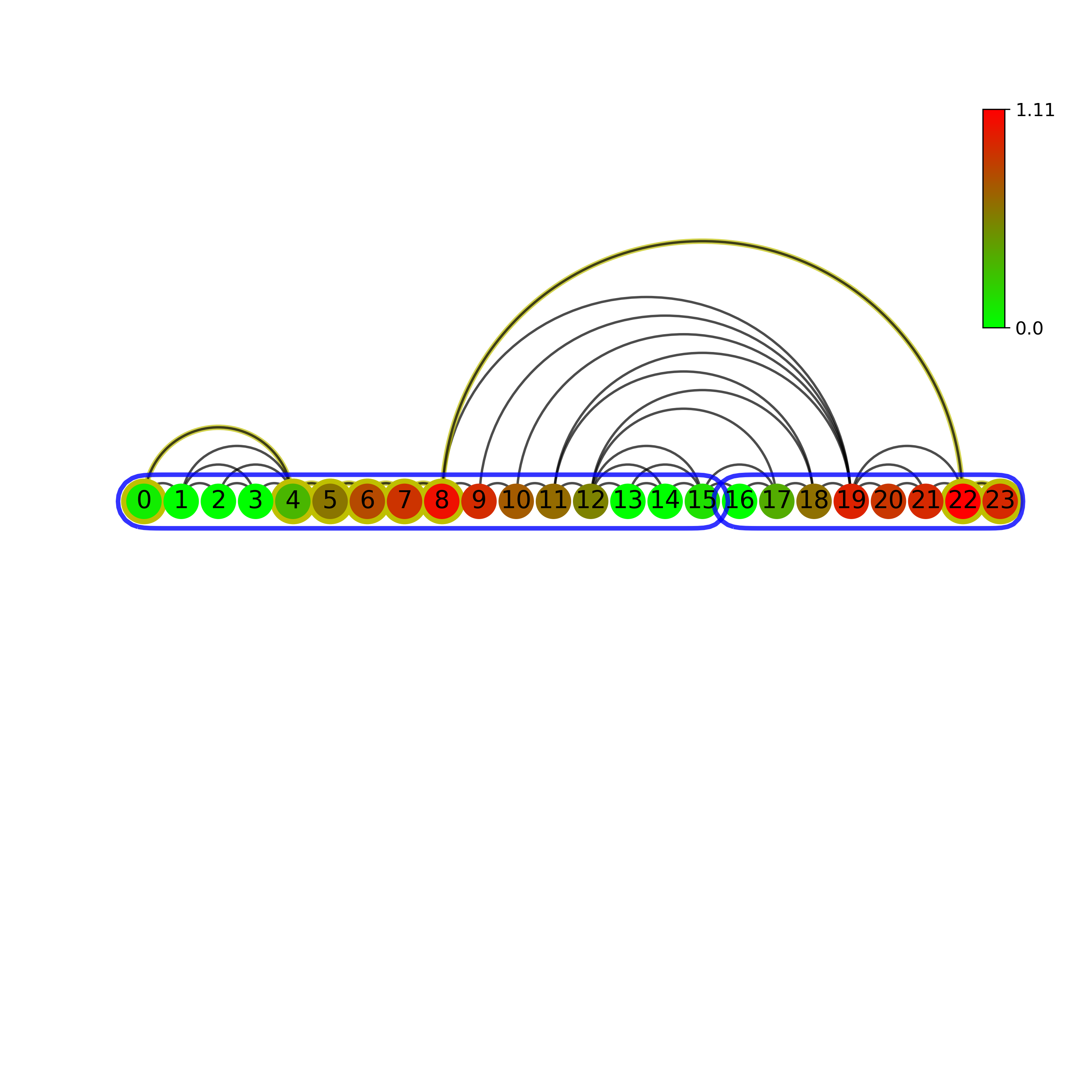
Normal (left) and Horizontal (right) bar-style visibility graph:
Visibility Graph Community Detection
import numpy as np
import networkx as nx
import pyiomica as pio
from pyiomica import visualizationFunctions
from pyiomica import visibilityGraphCommunityDetection
import matplotlib.pyplot as plt
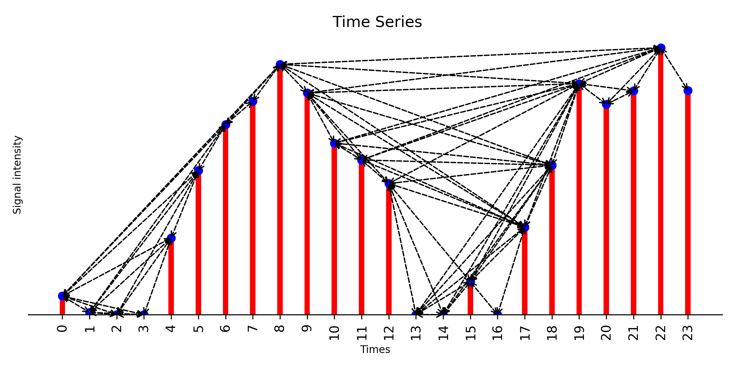
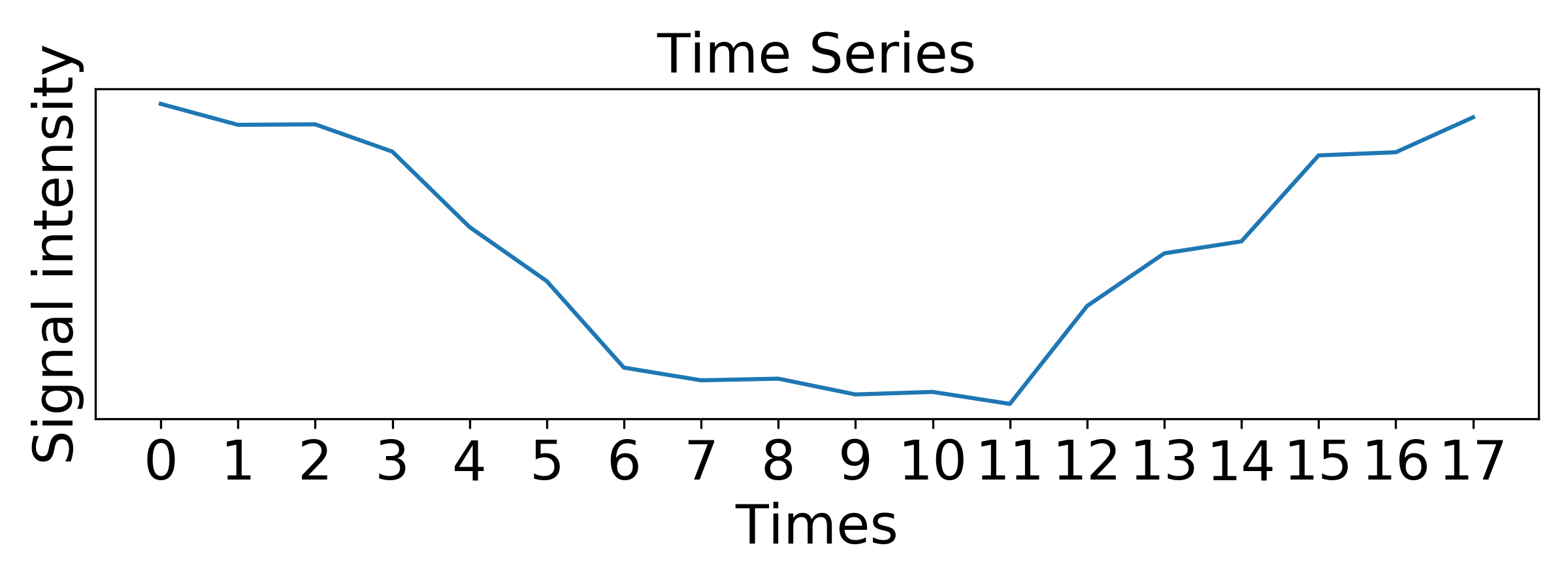
### create time series
np.random.seed(11)
times = np.arange( 0, 2*np.pi, 0.35)
tp = list(range(len(times)))
data = 5*np.cos(times) + 2*np.random.random(len(times))
### plot time series
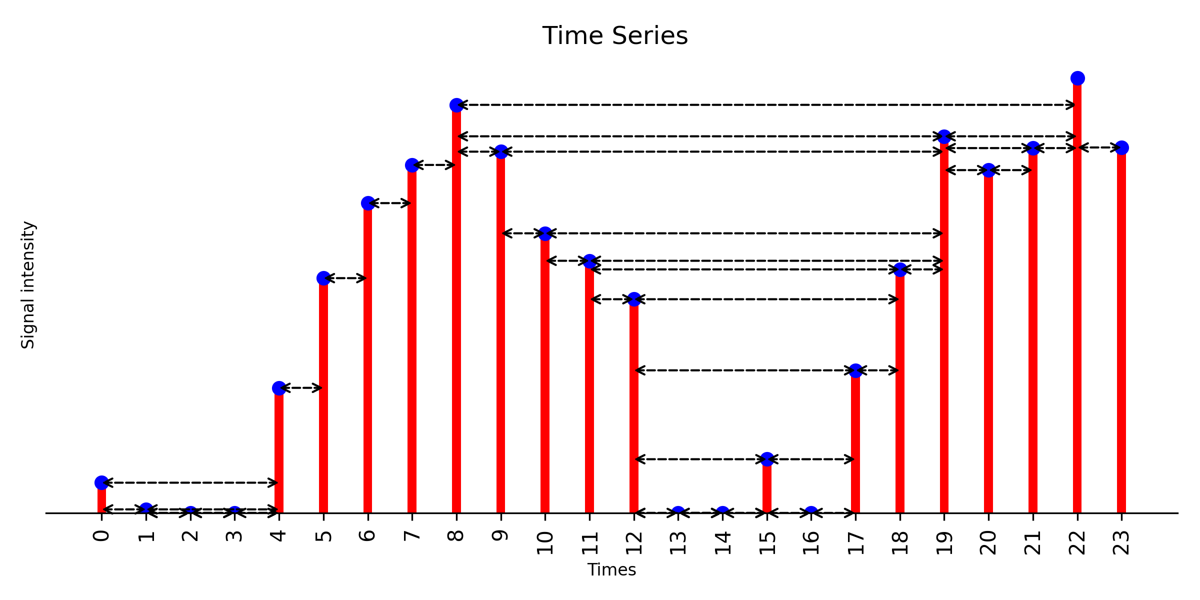
fig, ax = plt.subplots(figsize=(8,3))
ax.plot(tp,data)
ax.set_title('Time Series', fontdict={'color': 'k'},fontsize=20)
ax.set_xlabel('Times', fontsize=20)
ax.set_ylabel('Signal intensity', fontsize=20)
ax.set_xticks(tp)
ax.set_xticklabels([str(item) for item in np.round(tp,2)],fontsize=20, rotation=0)
ax.set_yticks([])
fig.tight_layout()
filename ='./Time_series_graph.png'
fig.savefig(filename, dpi=300)
plt.close(fig)
### plot weighted natural visibility graph, weight is Euclidean distance
g_nx_NVG, A_NVG = visibilityGraphCommunityDetection.createVisibilityGraph(data, tp, "natural", weight = 'distance')
filename = './Natural_Visibility_Graph.png'
visualizationFunctions.plotNVGBarGraphDual(A_NVG, data, tp,fileName = filename,
title ='Natural Visibility Graph', fontsize=20, figsize=(8,3), dpi=300)
### plot reflected perspective weighted natural visibility graph, weight is Euclidean distance
g_nx_revNVG, A_revNVG = visibilityGraphCommunityDetection.createVisibilityGraph(-data, tp, "natural", weight = 'distance')
filename = './Reflected_perspective_Natural_Visibility_Graph.png'
visualizationFunctions.plotNVGBarGraphDual(A_revNVG, -data, tp, fileName = filename,
title='Reflected perspective Natural Visibility Graph', fontsize=20, figsize=(8,3), dpi=300)
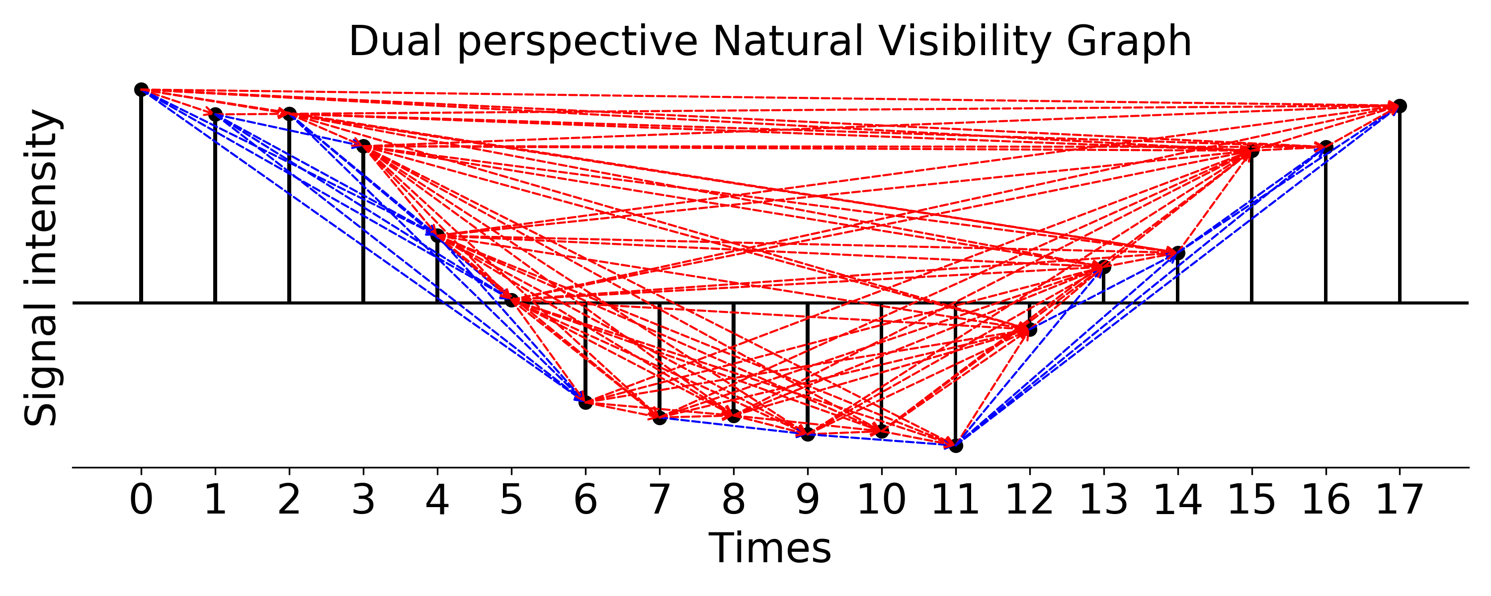
### plot dual perspective natural visibility graph, weight is Euclidean distance
g_nx_dualNVG, A_dualNVG = visibilityGraphCommunityDetection.createVisibilityGraph(data, tp, "dual_natural",
weight='distance', withsign=True)
filename = './Dual_perspective_Natural_Visibility_Graph.png'
visualizationFunctions.plotNVGBarGraphDual(A_dualNVG, data, tp, fileName=filename,
title='Dual perspective Natural Visibility Graph', fontsize=20, figsize=(10,4), dpi=300)
### plot line layout dual perspective natural visibility graph with community structure, weight is Euclidean distance
communities = visibilityGraphCommunityDetection.communityDetectByPathLength(g_nx_dualNVG, direction=None, cutoff='auto')
com = (communities, g_nx_dualNVG)
visualizationFunctions.makeVisibilityGraph(data, tp, './', 'Communities_of_Visibility_Graph', layout='line',communities=com,
level=0.8, figsize=(10,6), extension='png', dpi=300)
Extended DataFrame
Usage of some of the functions added to a standard DataFrame.
#import sys
#sys.path.append("../..")

# Import PyIOmica
import pyiomica as pio

# Import Extended DataFrame from PyIOmica
from pyiomica.extendedDataFrame import DataFrame

# Create a simple data for testing and demonstration
df_data = DataFrame(data=pio.np.array([[0.5,2,3],
                                      [0,2,6],
                                      [7,3,0],
                                      [2,2,8],
                                      [1,pio.np.nan,pio.np.nan],
                                      [6,0,0],
                                      [0,0,0],
                                      [3,3,3.1],
                                      [3,2,pio.np.nan],
                                      [4,pio.np.nan,4]]).astype(float),
                    index=['s1','s2','s3','s4','s5','s6','s7','s8','s9','s10'],
                    columns=['c1', 'c2', 'c3'])
print(df_data, '\n')

# Remove all-zero signals from the data
df_data.filterOutAllZeroSignals(inplace=True)
print(df_data, '\n')

# Remove firt-point-zero signals from the data
df_data.filterOutReferencePointZeroSignals(inplace=True)
print(df_data, '\n')

# Remove nearly-constant signals from the data
df_data.removeConstantSignals(0.2, inplace=True)
print(df_data, '\n')

# Remove signals with >75% non-zero points
df_data.filterOutFractionZeroSignals(0.6, inplace=True)
print(df_data, '\n')

# Remove signals with >75% non-zero points
df_data.filterOutFractionMissingSignals(0.8, inplace=True)
print(df_data, '\n')

# Add a signal with zeros
df_data.loc['s11'] = [2,0,6]
print(df_data, '\n')

# Replace any zeros with np.NaN (missing)
df_data.tagValueAsMissing(inplace=True)
print(df_data, '\n')

# Replace any missing values (np.NaN) with values
df_data.tagMissingAsValue(value=0, inplace=True)
print(df_data, '\n')

# Replace any values smaller than 'a' with 'b'
df_data.tagLowValues(1., 1., inplace=True)
print(df_data, '\n')

# Calculate modified zscore (median-based) of data
df_data_zm = df_data.modifiedZScore()
print(df_data_zm, '\n')

# Quantile normalize the data
df_data_qn = df_data.quantileNormalize()
print(df_data_qn, '\n')

# Box-cox transform data
df_data_bc = df_data.boxCoxTransform()
print(df_data_bc, '\n')

# Normalize signals to unity
df_data_un = df_data.normalizeSignalsToUnity()
print(df_data_un, '\n')
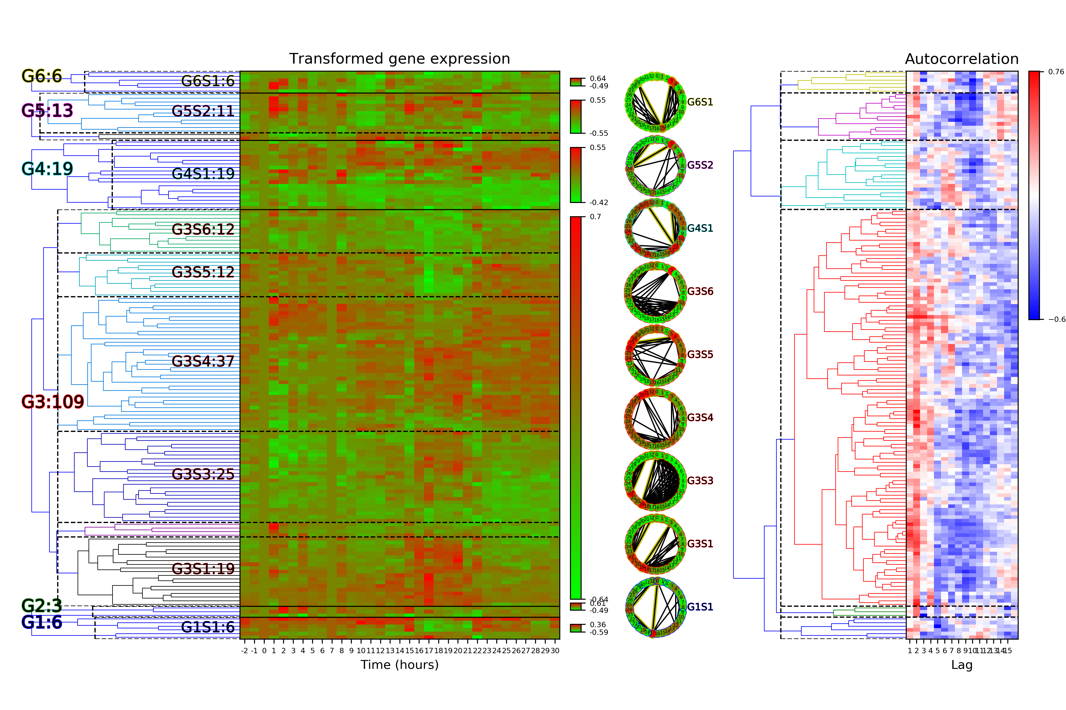
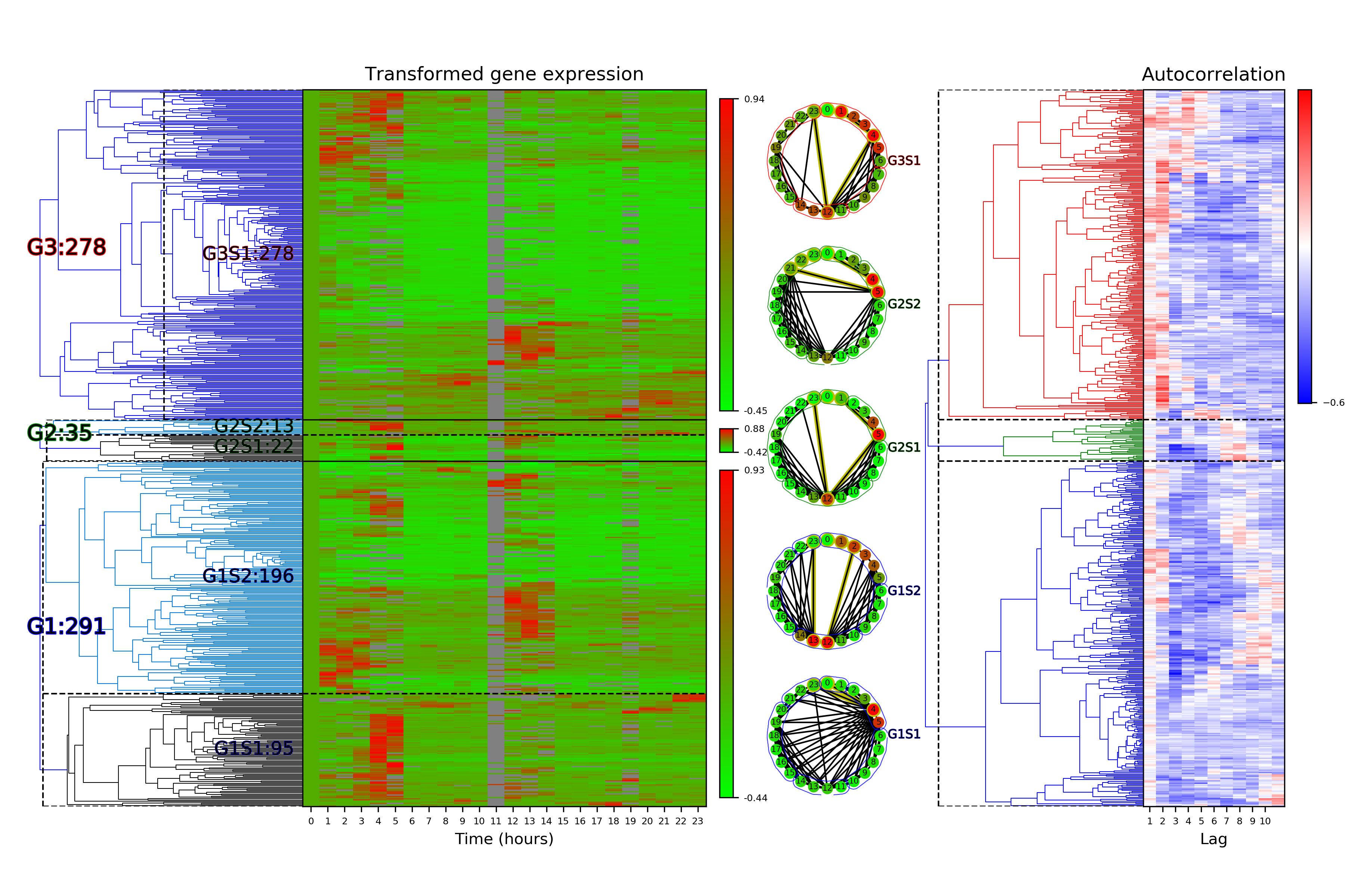
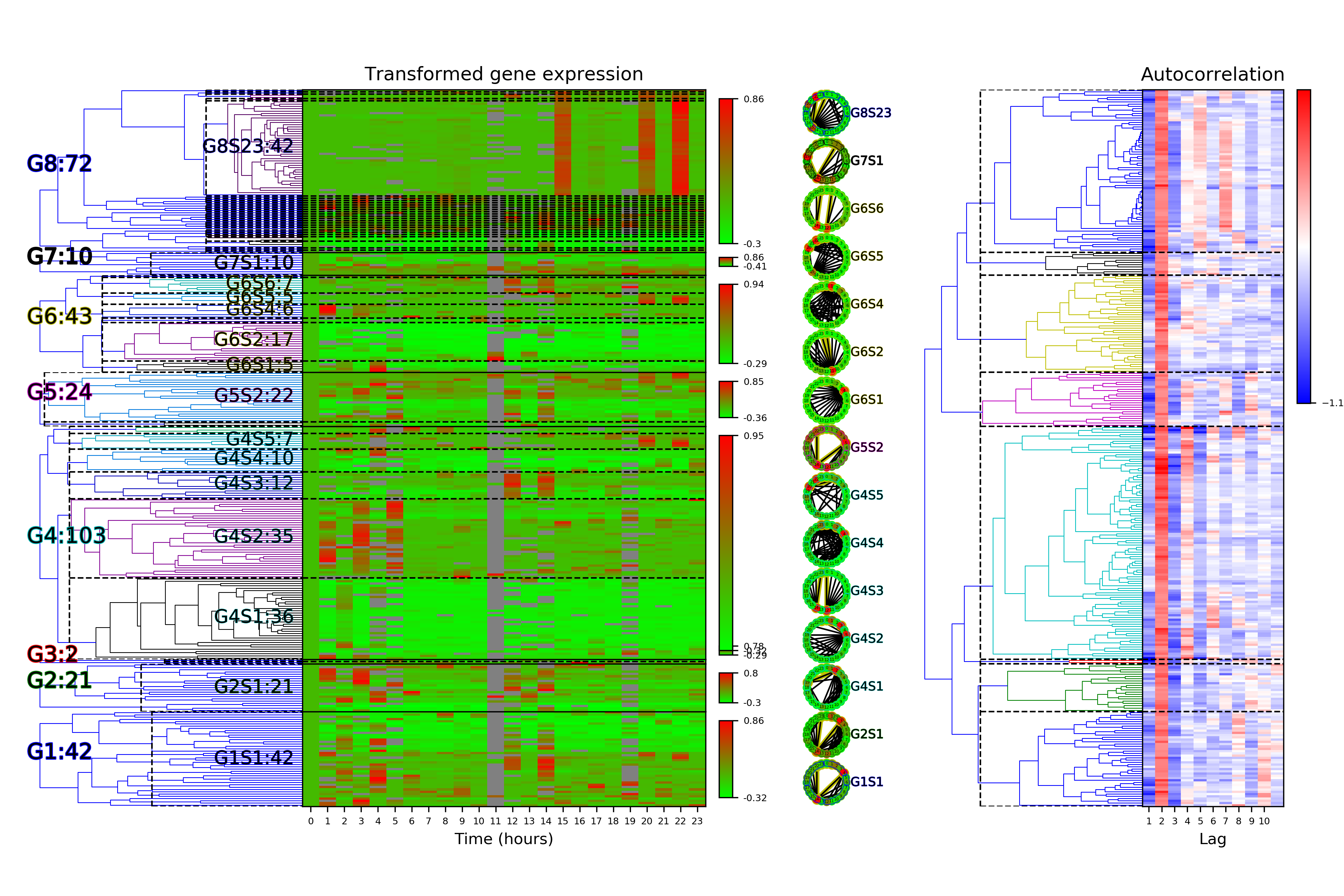
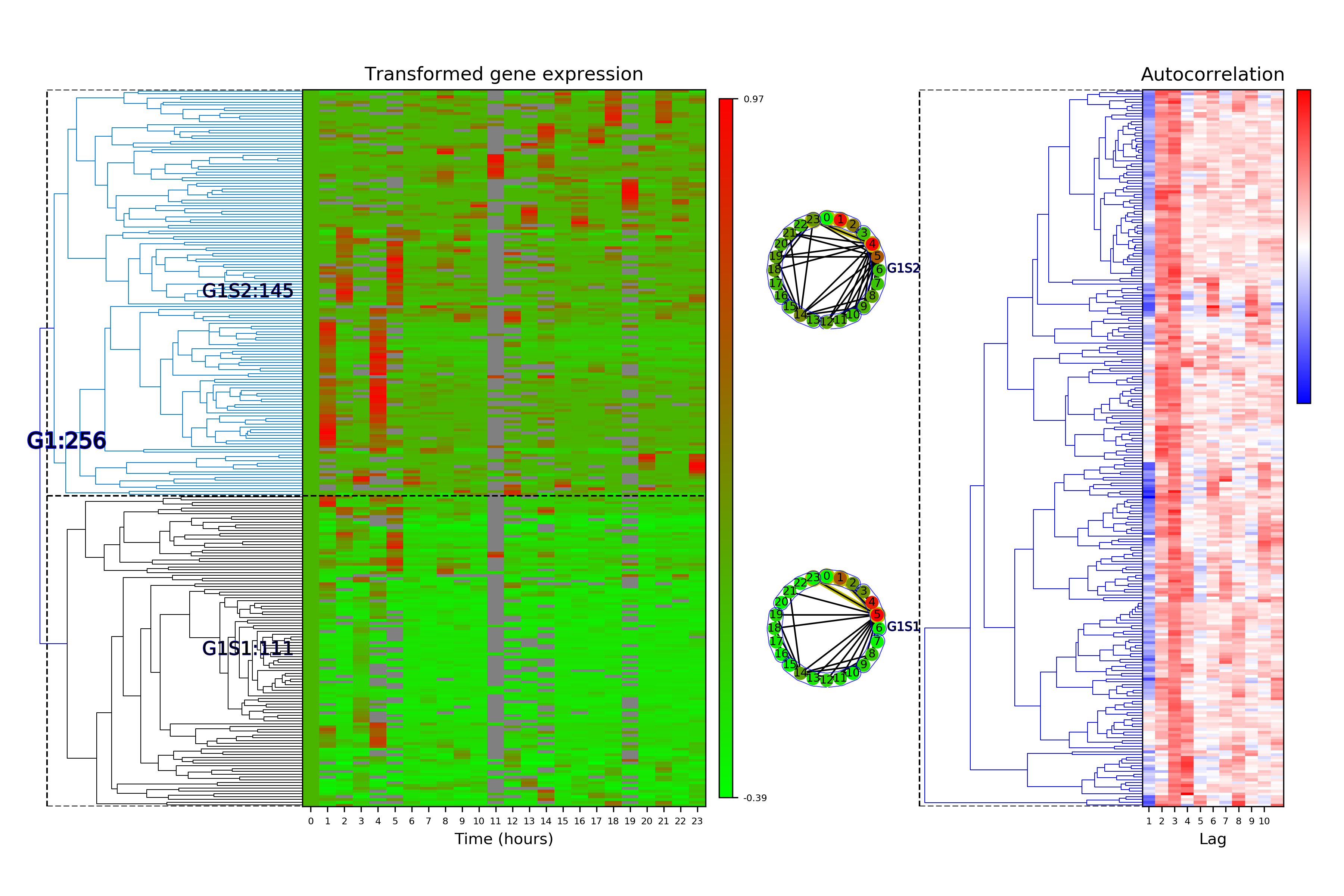
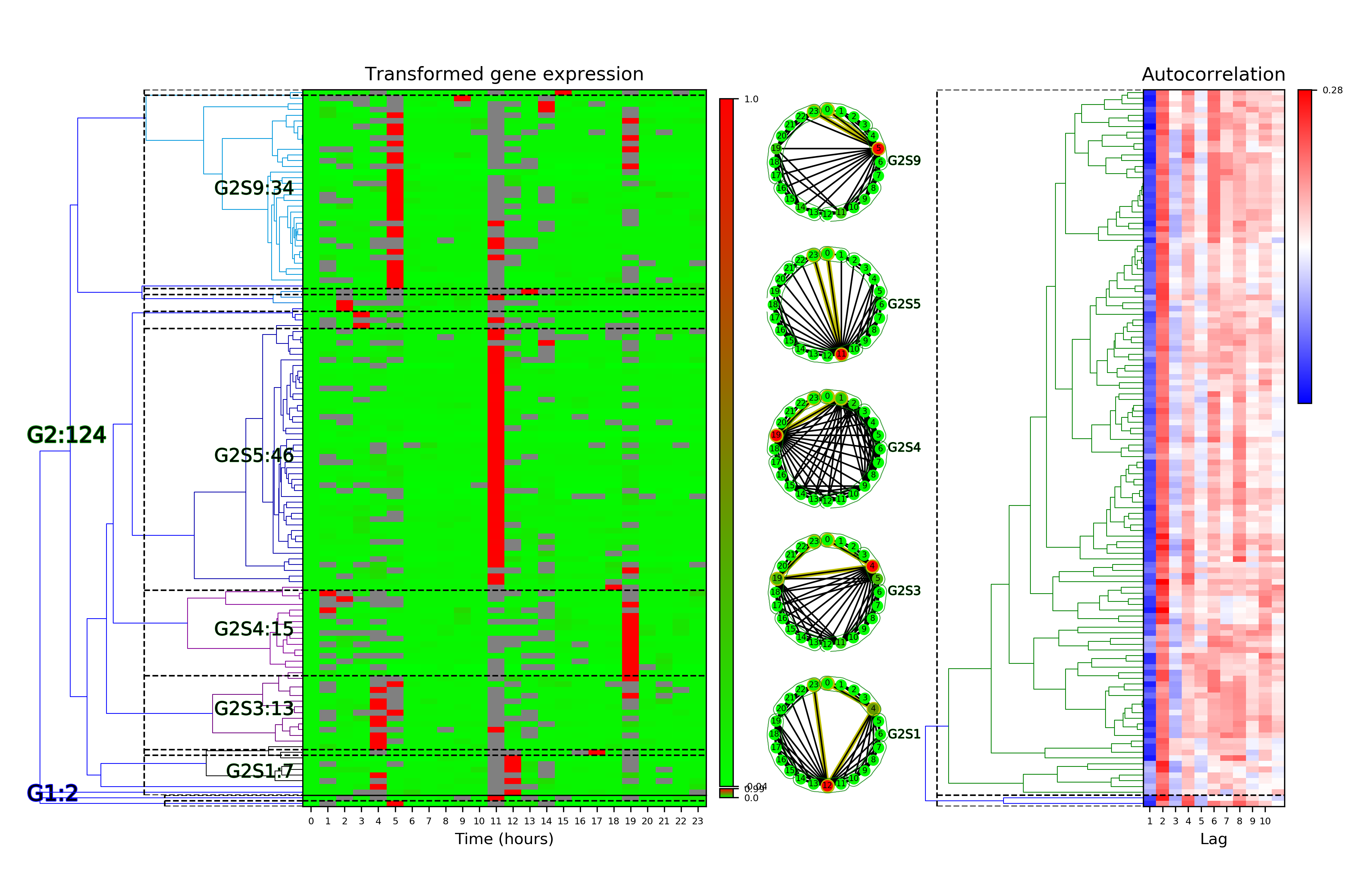
Time Series Categorization
#import sys
#sys.path.append("../..")
import pyiomica as pio
from pyiomica import categorizationFunctions as cf
if __name__ == '__main__':
# Unzip example data
with pio.zipfile.ZipFile(pio.os.path.join(pio.ConstantPyIOmicaExamplesDirectory, 'SLV.zip'), "r") as zipFile:
zipFile.extractall(path=pio.ConstantPyIOmicaExamplesDirectory)
# Process sample dataset SLV_Hourly1
# Name of the fisrt data set
dataName = 'SLV_Hourly1TimeSeries'
# Define a directory name where results are be saved
saveDir = pio.os.path.join('results', dataName, '')
# Directory name where example data is (*.csv files)
dataDir = pio.os.path.join(pio.ConstantPyIOmicaExamplesDirectory, 'SLV')
# Read the example data into a DataFrame
df_data = pio.pd.read_csv(pio.os.path.join(dataDir, dataName + '.csv'), index_col=[0,1,2], header=0)
# Calculate time series categorization
cf.calculateTimeSeriesCategorization(df_data, dataName, saveDir, NumberOfRandomSamples = 10**5)
# Cluster the time series categorization results
cf.clusterTimeSeriesCategorization(dataName, saveDir)
# Make plots of the clustered time series categorization
cf.visualizeTimeSeriesCategorization(dataName, saveDir)
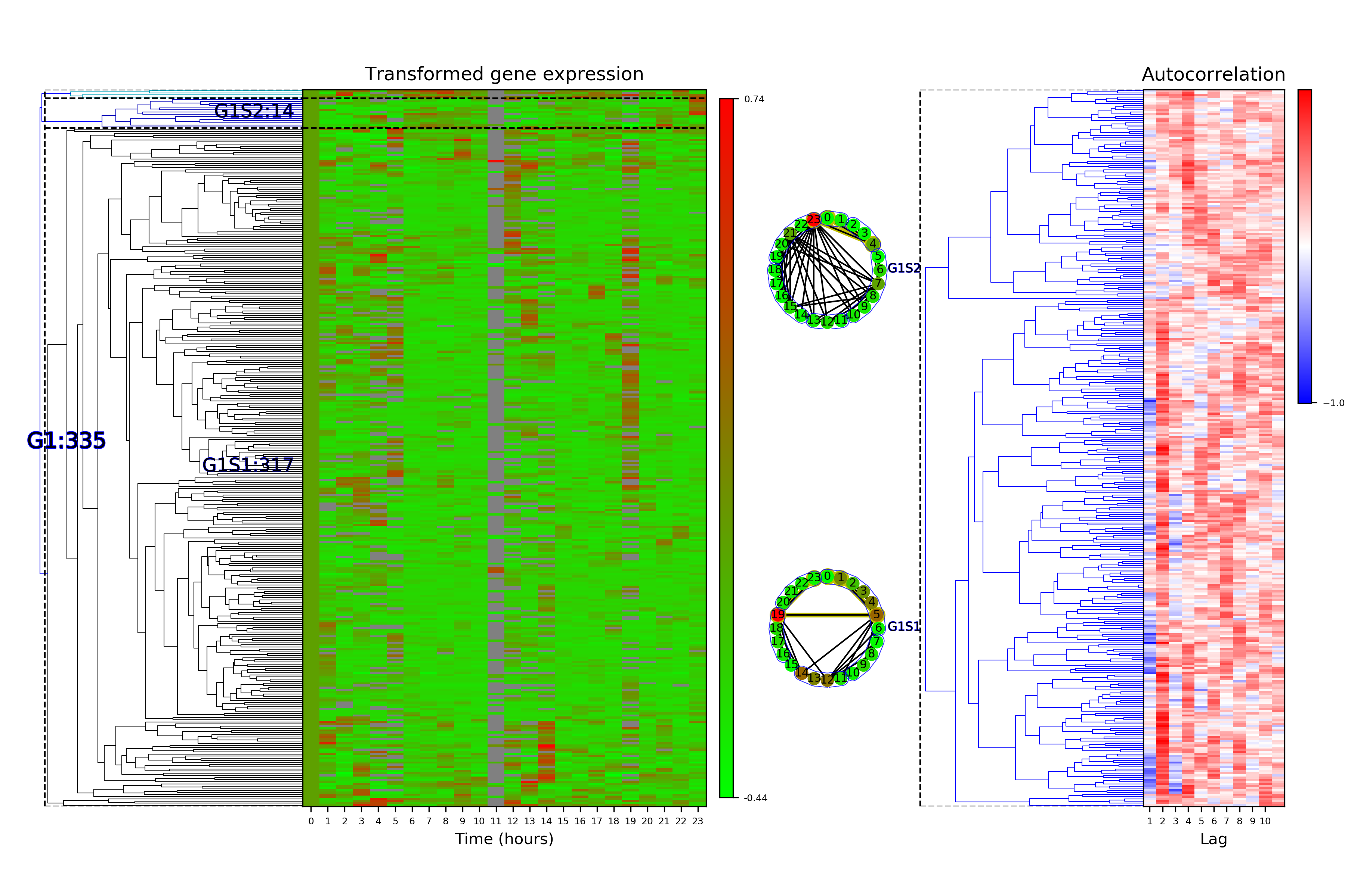
# Process sample dataset SLV_Hourly2, in the same way as SLV_Hourly1 above
dataName = 'SLV_Hourly2TimeSeries'
saveDir = pio.os.path.join('results', dataName, '')
dataDir = pio.os.path.join(pio.ConstantPyIOmicaExamplesDirectory, 'SLV')
df_data = pio.pd.read_csv(pio.os.path.join(dataDir, dataName + '.csv'), index_col=[0,1,2], header=0)
cf.calculateTimeSeriesCategorization(df_data, dataName, saveDir, NumberOfRandomSamples = 10**5)
cf.clusterTimeSeriesCategorization(dataName, saveDir)
cf.visualizeTimeSeriesCategorization(dataName, saveDir)
# Import data storage submodule to read results of processing sample datasets SLV_Hourly1 and SLV_Hourly2
from pyiomica import dataStorage as ds
# Use results from processing sample datasets SLV_Hourly1 and SLV_Hourly2 to calculate "Delta"
dataName = 'SLV_Hourly1TimeSeries'
df_data_processed_H1 = ds.read(dataName+'_df_data_transformed', hdf5fileName=pio.os.path.join('results',dataName,dataName+'.h5'))
dataName = 'SLV_Hourly2TimeSeries'
df_data_processed_H2 = ds.read(dataName+'_df_data_transformed', hdf5fileName=pio.os.path.join('results',dataName,dataName+'.h5'))
dataName = 'SLV_Delta'
saveDir = pio.os.path.join('results', dataName, '')
df_data = df_data_processed_H2.compareTwoTimeSeries(df_data_processed_H1, compareAllLevelsInIndex=False, mergeFunction=pio.np.median).fillna(0.)
cf.calculateTimeSeriesCategorization(df_data, dataName, saveDir, NumberOfRandomSamples = 10**5)
cf.clusterTimeSeriesCategorization(dataName, saveDir)
cf.visualizeTimeSeriesCategorization(dataName, saveDir)
#import sys
#sys.path.append("../..")

import pyiomica as pio

from pyiomica import categorizationFunctions as cf
from pyiomica import dataStorage as ds
from pyiomica import enrichmentAnalyses as ea

if __name__ == '__main__':

    # Unzip example data
    with pio.zipfile.ZipFile(pio.os.path.join(pio.ConstantPyIOmicaExamplesDirectory, 'SLV.zip'), "r") as zipFile:
        zipFile.extractall(path=pio.ConstantPyIOmicaExamplesDirectory)

    # Name of the fisrt data set
    dataName = 'DailyTimeSeries_SLV_Protein'

    # Define a directory name where results are be saved
    saveDir = pio.os.path.join('results', dataName, '')

    # Directory name where example data is (*.csv files)
    dataDir = pio.os.path.join(pio.ConstantPyIOmicaExamplesDirectory, 'SLV')

    # Read the example data into a DataFrame
    df_data = pio.pd.read_csv(pio.os.path.join(dataDir, dataName + '.csv'), index_col=[0,1], header=0)

    # Calculate time series categorization
    cf.calculateTimeSeriesCategorization(df_data, dataName, saveDir, NumberOfRandomSamples = 10**5, referencePoint=2, preProcessData=False)

    # Cluster the time series categorization results
    cf.clusterTimeSeriesCategorization(dataName, saveDir)

    # Make plots of the clustered time series categorization
    cf.visualizeTimeSeriesCategorization(dataName, saveDir)

    # Do enrichment GO and KEGG analysis on LAG1 results
    LAG1 = ds.read('results/DailyTimeSeries_SLV_Protein/consolidatedGroupsSubgroups/DailyTimeSeries_SLV_Protein_LAG1_Autocorrelations_GroupsSubgroups')
    ea.ExportEnrichmentReport(ea.GOAnalysis(LAG1), AppendString='GO_LAG1', OutputDirectory='results/DailyTimeSeries_SLV_Protein/')
    ea.ExportEnrichmentReport(ea.KEGGAnalysis(LAG1), AppendString='KEGG_LAG1', OutputDirectory='results/DailyTimeSeries_SLV_Protein/')