Categorization functions¶

Submodule pyiomica.categorizationFunctions

Example of use of a function described in this module:

 # import the package and its mudule Categorization functions
 import pyiomica as pio
 from pyiomica import categorizationFunctions as cf

 # Location of this example data
 dir = pio.ConstantPyIOmicaExamplesDirectory

 # Unzip sample data
 with pio.zipfile.ZipFile(pio.os.path.join(dir, 'SLV.zip'), "r") as zipFile:
     zipFile.extractall(path=dir)

 # Process sample dataset SLV Hourly 1
 dataName = 'SLV_Hourly1TimeSeries'
 saveDir = pio.os.path.join('results', dataName, '')
 dataDir = pio.os.path.join(dir, 'SLV')
 df_data = pio.pd.read_csv(pio.os.path.join(dataDir, dataName + '.csv'), index_col=[0,1,2], header=0)
 cf.calculateTimeSeriesCategorization(df_data, dataName, saveDir, NumberOfRandomSamples = 10**4)
 cf.clusterTimeSeriesCategorization(dataName, saveDir)
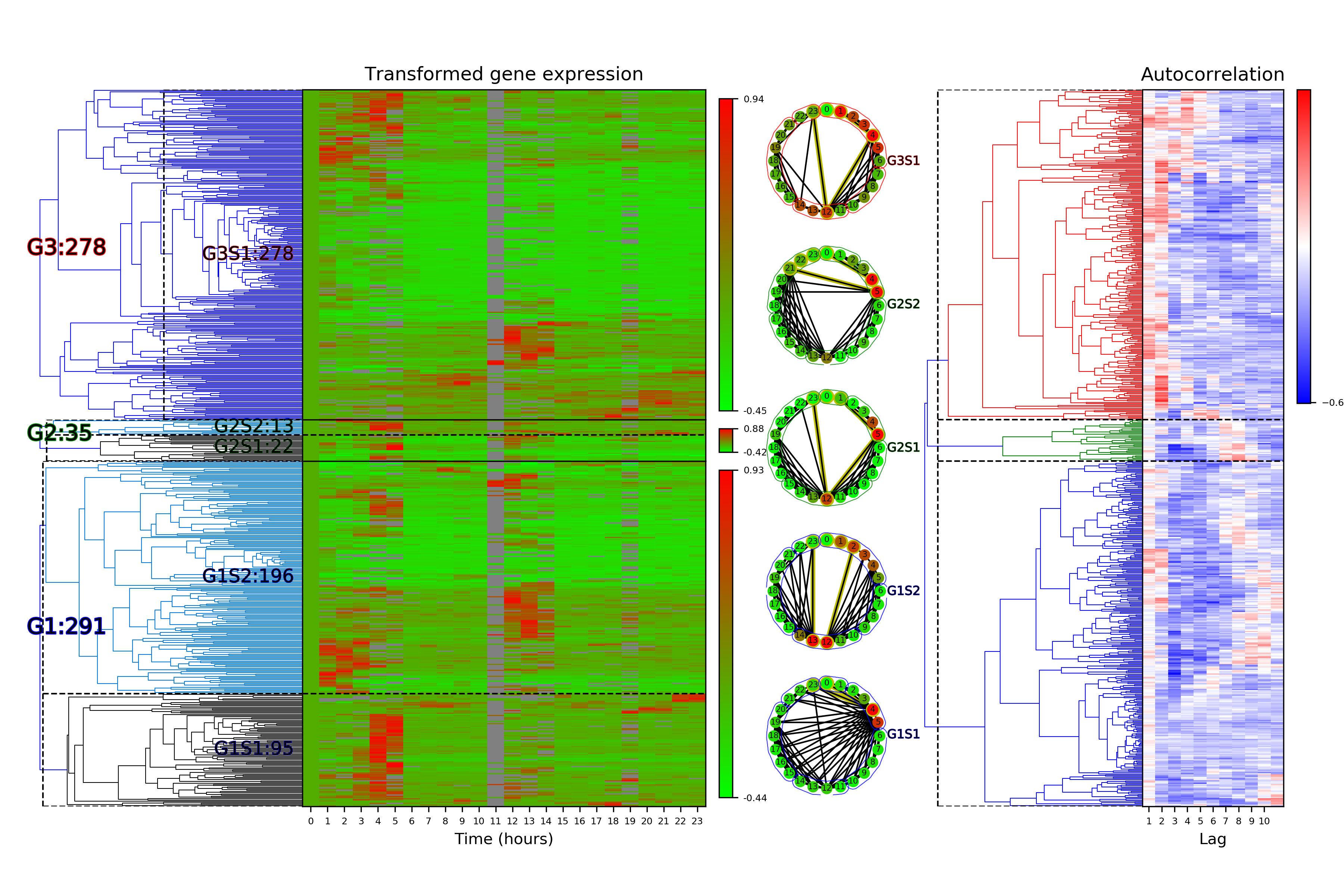
 cf.visualizeTimeSeriesCategorization(dataName, saveDir)

One of the figures generated by visualizeTimeSeriesCategorization is shown below:

Categorization functions

Functions:

`calculateTimeSeriesCategorization`(df_data, ...)	Time series classification.
`clusterTimeSeriesCategorization`(dataName, ...)	Visualize time series classification.
`visualizeTimeSeriesCategorization`(dataName, ...)	Visualize time series classification.

calculateTimeSeriesCategorization(df_data, dataName, saveDir, hdf5fileName=None, p_cutoff=0.05, fraction=0.75, constantSignalsCutoff=0.0, lowValuesToTag=1.0, lowValuesToTagWith=1.0, NumberOfRandomSamples=100000, NumberOfCPUs=4, referencePoint=0, autocorrelationBased=True, calculateAutocorrelations=False, calculatePeriodograms=False, preProcessData=True)[source]¶

Time series classification.

Parameters:

df_data: pandas.DataFrame: Data to process
dataName: str: Data name, e.g. “myData_1”
saveDir: str: Path of directories poining to data storage
hdf5fileName: str, Default None: Preferred hdf5 file name and location
p_cutoff: float, Default 0.05: Significance cutoff signals selection
fraction: float, Default 0.75: Fraction of non-zero point in a signal
constantSignalsCutoff: float, Default 0.: Parameter to consider a signal constant
lowValuesToTag: float, Default 1.: Values below this are considered low
lowValuesToTagWith: float, Default 1.: Low values to tag with
NumberOfRandomSamples: int, Default 10**5: Size of the bootstrap distribution to generate
NumberOfCPUs: int, Default 4: Number of processes allowed to use in calculations
referencePoint: int, Default 0: Reference point
autocorrelationBased: boolean, Default True: Whether Autocorrelation of Frequency based
calculateAutocorrelations: boolean, Default False: Whether to recalculate Autocorrelations
calculatePeriodograms: boolean, Default False: Whether to recalculate Periodograms
preProcessData: boolean, Default True: Whether to preprocess data, i.e. filter, normalize etc.

Returns:

None

Usage:

calculateTimeSeriesCategorization(df_data, dataName, saveDir)

clusterTimeSeriesCategorization(dataName, saveDir, numberOfLagsToDraw=3, hdf5fileName=None, exportClusteringObjects=False, writeClusteringObjectToBinaries=True, autocorrelationBased=True, method='weighted', metric='correlation', significance='Elbow')[source]¶

Visualize time series classification.

Parameters:

dataName: str: Data name, e.g. “myData_1”
saveDir: str: Path of directories pointing to data storage
numberOfLagsToDraw: int, Default 3: First top-N lags (or frequencies) to draw
hdf5fileName: str, Default None: HDF5 storage path and name
exportClusteringObjects: boolean, Default False: Whether to export clustering objects to xlsx files
writeClusteringObjectToBinaries: boolean, Default True: Whether to export clustering objects to binary (pickle) files
autocorrelationBased: boolean, Default True: Whether to label to print on the plots
method: str, Default ‘weighted’: Linkage calculation method
metric: str, Default ‘correlation’: Distance measure
significance: str, Default ‘Elbow’: Method for determining optimal number of groups and subgroups

Returns:

None

Usage:

clusterTimeSeriesClassification(‘myData_1’, ‘/dir1/dir2/’)

visualizeTimeSeriesCategorization(dataName, saveDir, numberOfLagsToDraw=3, autocorrelationBased=True, xLabel='Time', plotLabel='Transformed Expression', horizontal=False, minNumberOfCommunities=2, communitiesMethod='WDPVG', direction='left', weight='distance')[source]¶

Visualize time series classification.

Parameters:

dataName: str

Data name, e.g. “myData_1”

saveDir: str

Path of directories pointing to data storage

numberOfLagsToDraw: boolean, Default 3

First top-N lags (or frequencies) to draw

autocorrelationBased: boolean, Default True

Whether autocorrelation or frequency based

xLabel: str, Default ‘Time’

X-axis label

plotLabel: str, Default ‘Transformed Expression’

Label for the heatmap plot

horizontal: boolean, Default False

Whether to use horizontal or natural visibility graph.

minNumberOfCommunities: int, Default 2

Number of communities to find depends on the number of splits. This parameter is ignored in methods that automatically estimate optimal number of communities.

communitiesMethod: str, Default ‘WDPVG’

String defining the method to use for communitiy detection:

‘Girvan_Newman’: edge betweenness centrality based approach

‘betweenness_centrality’: reflected graph node betweenness centrality based approach

‘WDPVG’: weighted dual perspective visibility graph method (note to also set weight variable)

direction:str, default ‘left’

The direction that nodes aggregate to communities:

None: no specific direction, e.g. both sides.

‘left’: nodes can only aggregate to the left side hubs, e.g. early hubs

‘right’: nodes can only aggregate to the right side hubs, e.g. later hubs

weight: str, Default ‘distance’

Type of weight for communitiesMethod=’WDPVG’:

None: no weighted

‘time’: weight = abs(times[i] - times[j])

‘tan’: weight = abs((data[i] - data[j])/(times[i] - times[j])) + 10**(-8)

‘distance’: weight = A[i, j] = A[j, i] = ((data[i] - data[j])**2 + (times[i] - times[j])**2)**0.5

Returns:

None

Usage:

visualizeTimeSeriesClassification(‘myData_1’, ‘/dir1/dir2/’)